


The real story of stagflation has been saved
Cover image by: Jaime Austin

“Stagflation,” a word that became popular in the 1960s and 1970s, suggests that two things—inflation and high or rising unemployment—are happening at once.
The word first become popular (and was possibly first used) in reference to the British economy in the mid-1960s. The 1969 recession brought it across the Atlantic to the United States, as the Fed’s attempt to slow the economy resulted in a recession while inflation remained high. But the term, as carefully defined, appears to really have occurred only for short periods of time, despite what any memories of the 1970s might suggest.
With the term once again popping up in public discourse, it’s probably worthwhile to examine what it meant in the past, and what it might mean in the future.
Economic policy after World War II assumed that there was a trade-off between inflation and unemployment—the famous “Phillips curve.” William Phillips, an economist at the London School of Economics in the 1950s, noticed that periods of high inflation coincided with low unemployment.1 The idea intrigued many economists at the time, who interpreted the relationship as creating a trade-off.2 Policymakers, according to this view, could choose to accept lower unemployment at the expense of higher inflation. However, the attempt to actually use this concept resulted, in about a decade, in the United States’ first experience with stagflation.
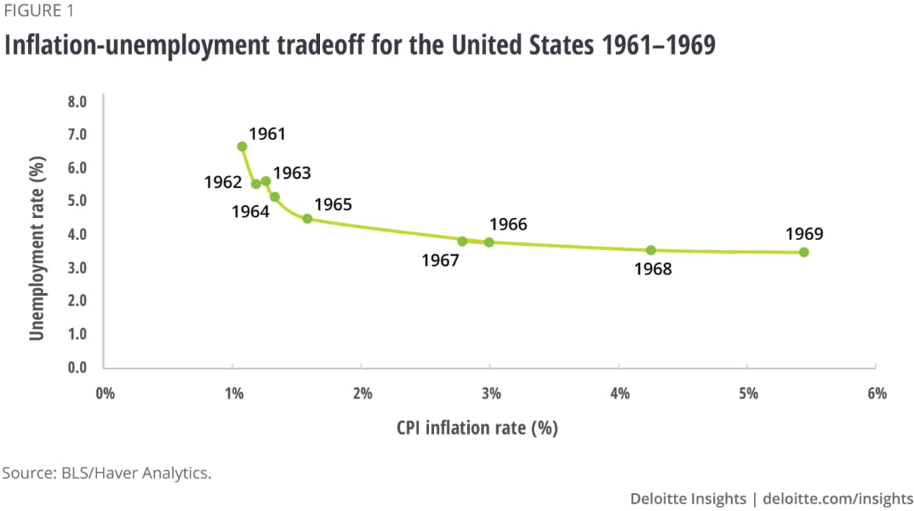
Figure 1 shows the Phillips curve for the United States using data from the 1960s. Notice the clear relationship over about 10 years—the higher inflation rates of the later years are (as expected) associated with lower unemployment rates. Up to this point, the Phillips curve analysis appeared correct, and the only real question was whether lower unemployment was worth the cost of higher inflation.
However, in 1969, the Fed embarked on a tightening cycle. Unemployment rose substantially in 1970, from 3.5% to 5.0%. But inflation actually accelerated in 1970 about half a percentage point, contrary to what the Phillips curve trade-off predicted. Instead of simply choosing a new point with lower inflation and unemployment, the economy experienced higher unemployment and higher inflation.
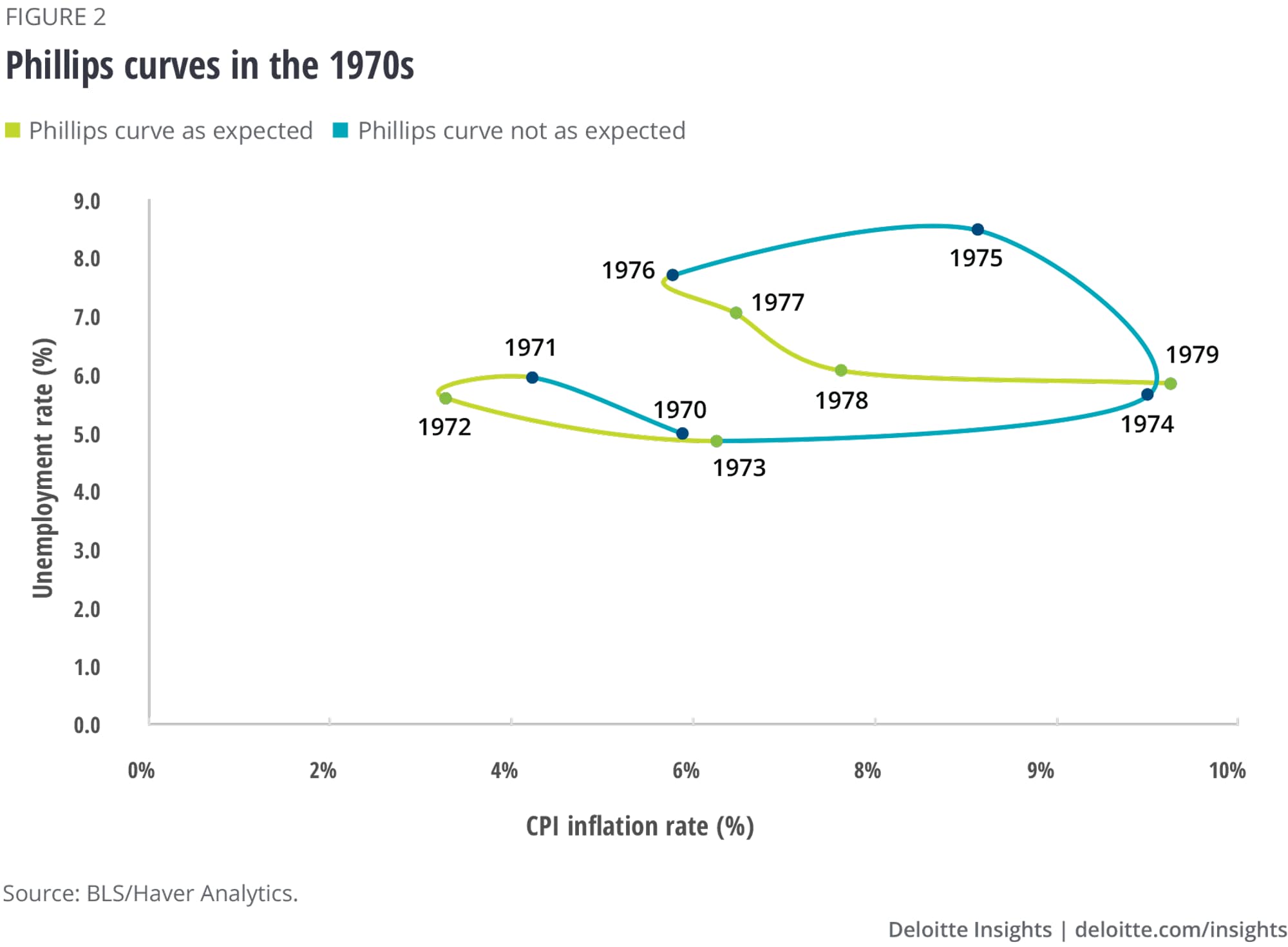
The 1970s saw more experiences like this (figure 2). The Phillips curve trade-off shows up in the 1971–73 period, as higher inflation is once again associated with lower unemployment. But the trade-off disappears over 1974–76, and only reappears in the last years of the decade. Years like 1971 and 1975 saw rising unemployment and rising inflation—the combination that characterizes stagflation.
And in the 1970s, the inflation rate associated with a given unemployment rate was higher than it was in the 1960s. In 1962, a relatively high unemployment rate of 5.6% was associated with an inflation rate of about 1%. In 1979, a 5.9% unemployment rate accompanied an 11% inflation rate. The Phillips curve shifted after the 1969–70 recession and then again after the 1973–1975 recession. Each time, a higher rate of inflation was associated with a given unemployment rate. It seemed as though each attempt by policymakers to exploit the Phillips curve trade-off shifted the curve farther to the right of the chart.
To understand why the Phillips curve shifted, it’s important to remember that the world is not like the ideal markets of economists’ imagination. In that world, prices adjust instantly to changes in the environment. In reality, businesses, consumers, and workers take time to decide to change prices, and must negotiate new prices with counterparties. When unemployment rises, both businesses and workers must take time to decide that wages need to soften and workers, of course, need to be convinced to accept wages that are losing purchasing power because of inflation. And it takes time for corporate executives to register that a fall in sales needs the response of lower prices. This process can take many months. That’s why there is a period when the inertia of past inflation keeps inflation high even as markets soften. And that’s why, as we see in the recessions of the 1970s, the downturn is accompanied by continued high or even rising inflation, despite the prediction of the Phillips curve.
That makes stagflation, in the strict sense, a short-term phenomenon. Once the economy begins to recover, the more usual relationship between unemployment and inflation asserts itself, although with (perhaps) a different level of expected inflation. Despite memories of stagflation in the 1970s, the last half of that decade saw inflation rising, but only as unemployment fell. That’s not stagflation—it’s the normal operation of the Phillips curve, only, as we’ve seen, at a higher level than the 1960s Phillips curve.
The big difference between the 1960s and the late 1970s is that workers and businesses had experienced higher inflation for some time in the 1970s. They therefore expected inflation to continue to be higher—and wage contracts and price-setting were done with higher inflation in mind.
In very high inflation economies, this process becomes automatic, as “cost of living allowances” (COLAs) are set to the government’s inflation data, removing the guesswork in expectations. This is sometimes called “indexation” of the economy. The United States never reached that point in the 1970s (although COLAs did become more common in some industries).
In this sense, inflation became baked into the economy. The result was a world in which relatively high (if falling) unemployment rates were associated with what appeared to be high inflation. But to repeat: Rising inflation was still associated with falling unemployment. There was never a long period of time when inflation and unemployment rose at the same time.
By 1979, dissatisfaction with high inflation created conditions for policymakers to try to reduce the baked-in level of inflation. Policymakers decided to try to reduce expectations by adopting restrictive monetary policies, slowing the economy, and (with an expected lag) reducing expectations. It is very unlikely that Paul Volcker, who shepherded the economy through the punishing recession that first began to bring inflation expectations down, Jimmy Carter, who appointed Volcker, or Ronald Reagan, who supported those efforts, expected the cost to be so high. But they did understand that something needed to be done to break the rise in inflationary expectations.3
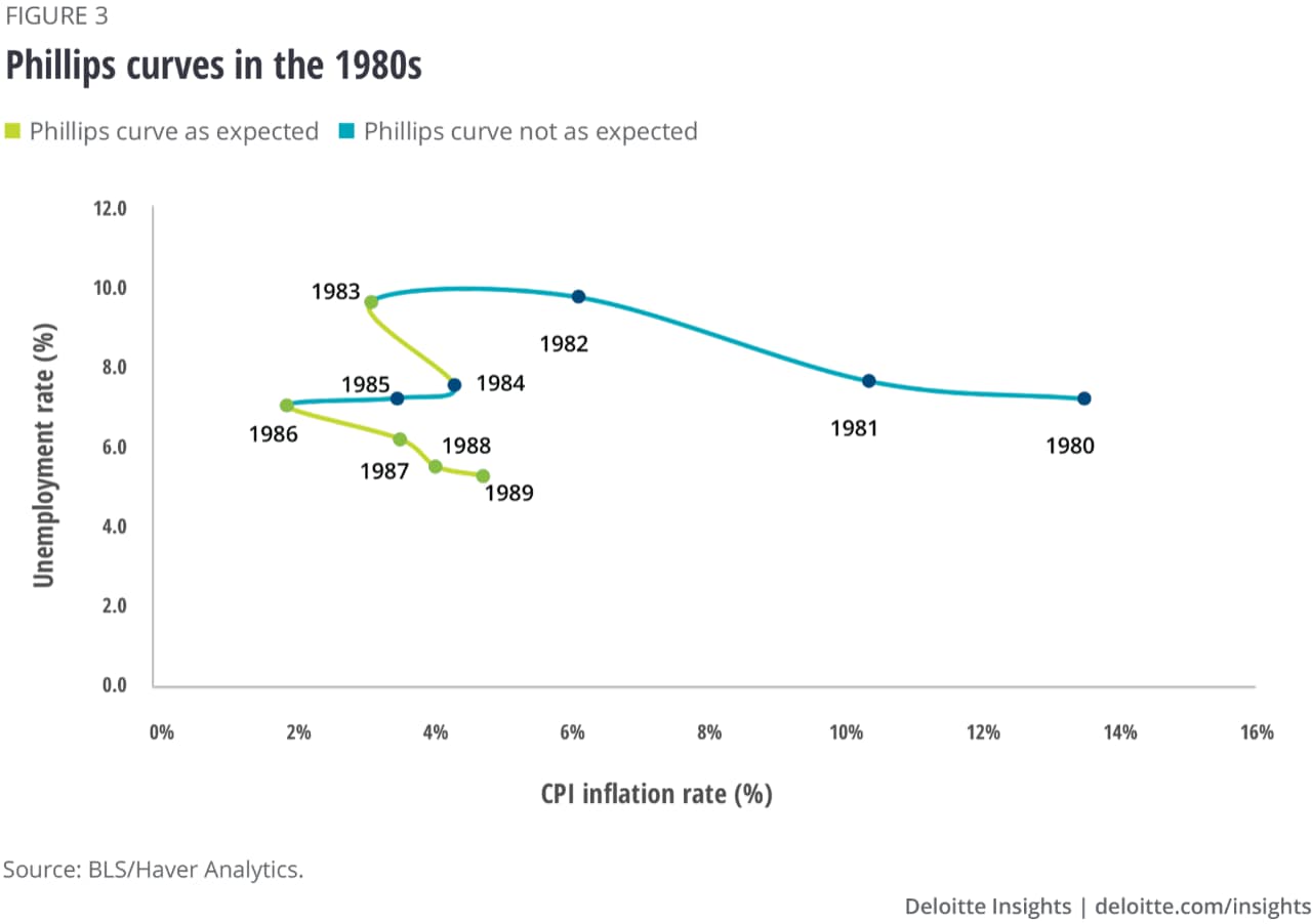
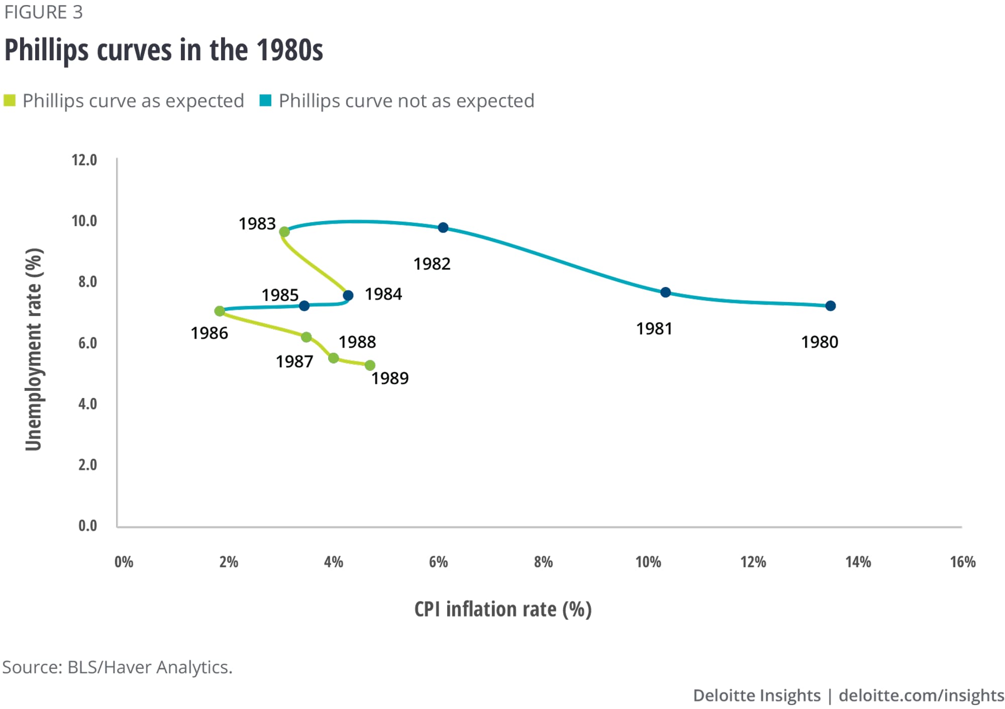
Figure 3 shows the Phillips curve relationship for the 1980s. Notice that Paul Volcker’s Fed rode the Phillips curve back up, initially lowering inflation by raising unemployment (during 1981–1983). In the mid-1980s, the inflation rate fell without any additional rise in unemployment (apparently a free lunch, although the actual payment was made in the earlier years), as expectations declined. It was the reverse of stagflation, and certainly welcome. By the late 1980s, a new Phillips curve with lower inflation rates for a given unemployment rate can be discerned.4
Stagflation in the pure sense of rising unemployment and high or rising inflation, therefore, is a temporary phenomenon. The economy typically encounters stagflation during recessions or significant slowdowns, and it disappears as the economy recovers. But the economy may experience higher inflation at a given unemployment rate as expectations rise, and that might be seen as “stagflation.” The higher base inflation does not preclude the economy operating at full employment. But dissatisfaction with high inflation could impel policymakers to slow the economy—or even create a recession—to bring expectations back down to acceptable levels.
Currently, long-term inflation expectations appear to be “anchored” (in the Fed’s terminology). The 10-year Treasury break-even rate—the inflation rate implied by Treasury inflation-indexed securities—is at the same level as in the early 2010s, when inflation was hardly a concern. Economic forecasters, such as those in the Wall Street Journal Economic Forecasting survey or in the National Association for Business Economics Outlook survey, are projecting a decline in inflation next year.5 The Fed will continue to look carefully at how expectations evolve. But the bottom line is that, while a short period of stagflation (less than a year) may occur when the economy slows, a wholesale shifting of the Phillips curve does not appear to have occurred, keeping the cost of controlling inflation much lower than it was in the 1980s.
A.W. Phillips, “The relation between unemployment and the rate of change of money wage rates in the United Kingdom,” Economica 25, no. 100 (1958): pp. 283–299.
View in ArticleFor more background (if a bit more technical), please see: Robert J. Gordon, “The history of the Phillips curve: An American perspective,” keynote address, Australasian Meetings of the Econometric Society, July 9, 2008.
View in ArticleOddly enough, it is cheaper and easier to reduce expectations and stop inflation when it is very high. Please see: Thomas J. Sargent, “The end of four big inflations,” in Robert E. Hall, “Inflation, causes and effects,” University of Chicago Press, 1982, pp. 41–97. Israel provides a more modern example. Please see: Dany Bahar, “How Shimon Peres saved the Israeli economy,” Brookings, September 30, 2016.
View in ArticleBy the 1990s, and over the period up to the pandemic in 2020, the Phillips curve relationship appeared to have disappeared. That may simply be the result of the Fed’s policy keeping inflation steady rather than the nonexistence of a short-term trade-off. Economists are still trying to fully understand the “great moderation” of 1995–2019.
View in ArticleAnthony DeBarros, “About the Wall Street Journal Economic Forecasting survey,” Wall Street Journal, June 19, 2022; NABE, “NABE Outlook Survey,” May 2022.
View in ArticleCover image by: Jaime Austin